---
title: "The Mahalanobis distance"
description: >
The distance the other two methods are built on: why correlated columns are
counted once, how to handle categorical features, and where it fails
silently.
date: 2026-08-24
order: 3
categories: [distance, covariance]
image: thumbnail.png
jupyter: python3
---
```{python}
#| label: setup
#| include: false
import numpy as np
import matplotlib as mpl
import matplotlib.pyplot as plt
import pandas as pd
from scipy import stats
rng = np.random.default_rng(20260824)
mpl.rcParams.update({
"figure.facecolor": "white",
"axes.facecolor": "white",
"axes.edgecolor": "#b9c0c7",
"axes.linewidth": 0.9,
"axes.grid": True,
"axes.axisbelow": True,
"grid.color": "#e6e9ec",
"grid.linewidth": 0.8,
"axes.spines.top": False,
"axes.spines.right": False,
"axes.titlesize": 12,
"axes.titleweight": "semibold",
"axes.labelsize": 11,
"xtick.labelsize": 10,
"ytick.labelsize": 10,
"xtick.color": "#5b6570",
"ytick.color": "#5b6570",
"legend.frameon": False,
"legend.fontsize": 10,
"font.size": 11,
})
# A small, consistent palette used across every figure in the article.
C = {
"blue": "#2c6e9b",
"orange": "#d1743a",
"green": "#4f8f63",
"red": "#b5483d",
"grey": "#9aa3ab",
"dark": "#2c4a63",
}
```
The Mahalanobis distance centres, rescales, and removes correlation. We will
use it extensively to create balanced treatment and control groups with the
[Rerandomization](../rerandomization/) and
[Pairwise Matching](../pairwise-matching/) techniques.
It is worth knowing what the choice buys before working through it. Balancing
on covariate *means* only constrains the part of the outcome that is linear in
the covariates, while matching on this distance constrains any function of
them. In the [pairwise matching](../pairwise-matching/) article that difference
is the whole result: on an outcome the covariates predict well both designs are
worth about the same, and on one they predict just as strongly but non-linearly
the mean-based criterion collapses while matching holds its gain. The two
failure modes at the end of this article, a near-singular $\Sigma$ and a rare
categorical level, are the two ways that distance quietly stops measuring what
you think it measures.
For a point $x$, a mean vector $\mu$ and a covariance
matrix $\Sigma$, the **squared Mahalanobis distance** is
::: {.keybox}
$$
D^2(x;\mu,\Sigma) \;=\; (x-\mu)^{\!\top}\,\Sigma^{-1}\,(x-\mu).
$$
:::
If you recognise that as the term that depends on $x$ in the
multivariate normal density, skip the next box. If not, the box is for you.
::: {.callout-tip collapse="true"}
## New to this? Build the formula up from the z-score
Nothing here is needed later on; it is the same formula, arrived at slowly.
**One variable.** Suppose heights have mean $\mu = 170$ cm and standard
deviation $\sigma = 10$ cm. Someone 190 cm tall is 20 cm above average, which is
2 standard deviations. That is the **z-score**:
$$
z = \frac{x - \mu}{\sigma} = \frac{190 - 170}{10} = 2.
$$
The point of dividing by $\sigma$ is that it makes the number *unitless*, so
"2 standard deviations out" means the same thing for heights in centimetres and
for incomes in pounds. Squaring it gives an unsigned measure of unusualness:
$$
z^2 = \frac{(x-\mu)^2}{\sigma^2} = (x-\mu)\,(\sigma^2)^{-1}\,(x-\mu) .
$$
That last way of writing it looks perverse, but it shows the similarity to the
formula for the Mahalanobis distance: centre, divide by the variance, and
square.
The term $z^2$ appears in the normal density:
$$
f(x) = \frac{1}{\sqrt{2\pi\sigma^2}}
\exp\!\left(-\tfrac{1}{2}\,\frac{(x-\mu)^2}{\sigma^2}\right)
= \underbrace{\frac{1}{\sqrt{2\pi\sigma^2}}}_{\text{a constant}}
\exp\!\left(-\tfrac{1}{2} z^2\right).
$$
The only place $x$ appears at all is inside $z^2$. So the measure of how unusual
a point is depends only on $z^2$.
**Several variables.** Now each observation is a list of numbers, say
$x = (\text{age},\ \text{height},\ \text{weight})$, so $x$ and $\mu$ are
vectors with $p = 3$ entries.
The single variance $\sigma^2$ has to become something richer, because there are
now two kinds of information: how much each variable varies on its own, and
whether variables move together. It becomes the **covariance matrix**
$\Sigma$, a $p \times p$ matrix whose diagonal entry $\Sigma_{jj}$ is the
variance of variable $j$, and whose off-diagonal entry $\Sigma_{jk}$ is the
covariance between variables $j$ and $k$. The covariance is positive if they
tend to be large together, zero if they are unrelated.
We don't divide by a matrix, but multiply by its inverse. Now
$\Sigma^{-1}$ is the matrix that plays the role $1/\sigma^2$ played before.
(Note that for one variable, $\Sigma$ is the $1\times1$ matrix $[\sigma^2]$
and $\Sigma^{-1}$ is $[1/\sigma^2]$, so the one-variable case really is the
general case with $p = 1$.)
Make those two substitutions in $(x-\mu)(\sigma^2)^{-1}(x-\mu)$ and you get
$$
(x-\mu)^{\!\top}\,\Sigma^{-1}\,(x-\mu),
$$
where the $^{\top}$ ("transpose") turns the first column of numbers on its
side so the multiplication is legal. The result is a single number, not a
vector or a matrix.
The formula for the multivariate normal is:
$$
f(x) = \frac{1}{(2\pi)^{p/2}\,|\Sigma|^{1/2}}
\exp\!\left(-\tfrac{1}{2}\,(x-\mu)^{\!\top}\Sigma^{-1}(x-\mu)\right).
$$
Side by side:
| | one variable | several variables |
|--------------------------|-------------------------------------|------------------------------------------|
| deviation | $x - \mu$ (a number) | $x - \mu$ (a vector) |
| "divide by the variance" | $(\sigma^2)^{-1}$ | $\Sigma^{-1}$ (a matrix) |
| squared distance | $\dfrac{(x-\mu)^2}{\sigma^2}$ | $(x-\mu)^{\!\top}\Sigma^{-1}(x-\mu)$ |
| appears in the density as| $\exp(-\tfrac12 z^2)$ | $\exp(-\tfrac12 D^2)$ |
So the Mahalanobis distance is the squared z-score, generalised to several
variables at once, and the generalisation is forced, not chosen: it is
whatever has to sit in the exponent of the multivariate normal.
:::
## What the matrix product is doing
$\Sigma$ is symmetric and positive definite, so it has a symmetric square root
$\Sigma^{1/2}$, and $\Sigma^{-1} = \Sigma^{-1/2}\Sigma^{-1/2}$. Substituting
that in and regrouping:
$$
D^2 = (x-\mu)^{\!\top}\Sigma^{-1/2}\,\Sigma^{-1/2}(x-\mu)
= \big\|\,\underbrace{\Sigma^{-1/2}(x-\mu)}_{\textstyle w}\,\big\|^2 .
$$
::: {.keybox}
**The Mahalanobis distance is ordinary Euclidean distance, computed after
whitening.** Centre by $\mu$, apply $\Sigma^{-1/2}$, then measure length the
usual way.
:::
The transformed vector $w = \Sigma^{-1/2}(x - \mu)$ has mean $0$ and covariance
$\Sigma^{-1/2}\Sigma\Sigma^{-1/2} = I$. In $w$-coordinates every variable has
variance one and no two are correlated, so the cloud is a sphere, and Euclidean
distance is finally the right tool. In practice, we use a Cholesky factor
$\Sigma = LL^{\top}$ and $w = L^{-1}(x-\mu)$ instead of the symmetric root.
Drag the slider below to watch it happen. The dashed rings are contours of
constant Mahalanobis distance at every stage, so they begin as the data's own
tilted ellipses and end as true circles. The red segment marks one fixed
observation: its length on screen changes, its Mahalanobis distance does not.
```{python}
#| label: fig-whitening
#| classes: preview-image
import json, pathlib
from IPython.display import HTML, display
Sig_demo = np.array([[9.0, 7.2], [7.2, 16.0]])
mu_demo = np.array([50.0, 120.0])
cloud = rng.multivariate_normal(mu_demo, Sig_demo, size=400)
focus = np.array([54.0, 116.0]) # the observation we track
L = np.linalg.cholesky(Sig_demo)
d_raw = focus - mu_demo
payload = {
"pts": np.round(cloud - mu_demo, 3).tolist(), # centred cloud
"focus": np.round(d_raw, 6).tolist(),
"mu": mu_demo.tolist(),
"L": L.tolist(),
"Linv": np.linalg.inv(L).tolist(),
"Dval": float(np.sqrt(d_raw @ np.linalg.solve(Sig_demo, d_raw))),
# The grid and its labels carry the first half of the slider on their own
# (centring only changes the numbers) so they are drawn stronger here
# than in the static figures, where they are just background.
"colors": {"grey": C["grey"], "red": C["red"], "dark": C["dark"],
"grid": "#ccd4db", "axis": "#9aa4ad", "tick": "#3f4850"},
}
js = pathlib.Path("whitening-widget.js").read_text(encoding="utf-8")
js = js.replace("__ID__", "mw-whiten").replace("__DATA__", json.dumps(payload))
display(HTML("""
<style>
.mahal-widget { margin: 1.2rem 0 1.6rem; }
.mahal-widget canvas { display:block; width:100%; touch-action:manipulation; }
.mahal-widget .mw-readout { font-size:.82rem; color:#5b6570; text-align:center;
margin:.35rem 0 .7rem; }
.mahal-widget .mw-readout b { color:#21252b; font-variant-numeric:tabular-nums; }
.mahal-widget .mw-sep { margin:0 .6rem; opacity:.45; }
.mahal-widget input[type=range] { width:100%; margin:0; accent-color:#2c6e9b; }
/* A native range input insets its thumb by half a thumb width at each end,
so pad the label row to match. Without this the thumb at minimum sits ~9px
to the right of where "raw x" begins. */
.mahal-widget .mw-labels { display:flex; justify-content:space-between;
font-size:.82rem; color:#8a929a; margin-top:.3rem; padding:0 9px;
/* fig-align:center puts text-align:center on the figure wrapper, which
would centre the first label inside its own column. Reset it here. */
text-align:left; }
.mahal-widget .mw-labels span { cursor:pointer; flex:1; text-align:left; }
.mahal-widget .mw-labels span:nth-child(2) { text-align:center; }
.mahal-widget .mw-labels span:nth-child(3) { text-align:right; }
.mahal-widget .mw-labels span.mw-on { color:#2c4a63; font-weight:600; }
</style>
<div class="mahal-widget" id="mw-whiten">
<canvas></canvas>
<div class="mw-readout"></div>
<input type="range" min="0" max="1000" step="1" value="0"
aria-label="Transformation: raw, centred, or whitened">
<div class="mw-labels">
<span data-at="0">raw <i>x</i></span>
<span data-at="500">centred <i>x</i> − <i>μ</i></span>
<span data-at="1000">whitened <i>L</i>⁻¹(<i>x</i> − <i>μ</i>)</span>
</div>
</div>
<script>""" + js + "</script>"))
```
## Three columns, two of them correlated
Let's think about a realistic example. Take $X$ with three columns:
`age`, `height_cm`, `weight_kg`, where height and weight are correlated at
$0.7$ and age is uncorrelated with both.
```{python}
#| label: example-setup
names = ["age", "height_cm", "weight_kg"]
mu_x  = np.array([50.0, 170.0, 75.0])
sd_x  = np.array([12.0,  10.0,  15.0])
R_x   = np.array([[1.0, 0.0, 0.0],
                  [0.0, 1.0, 0.7],
                  [0.0, 0.7, 1.0]])
S_x   = np.outer(sd_x, sd_x) * R_x          # covariance = D R D
S_inv = np.linalg.inv(S_x)
```
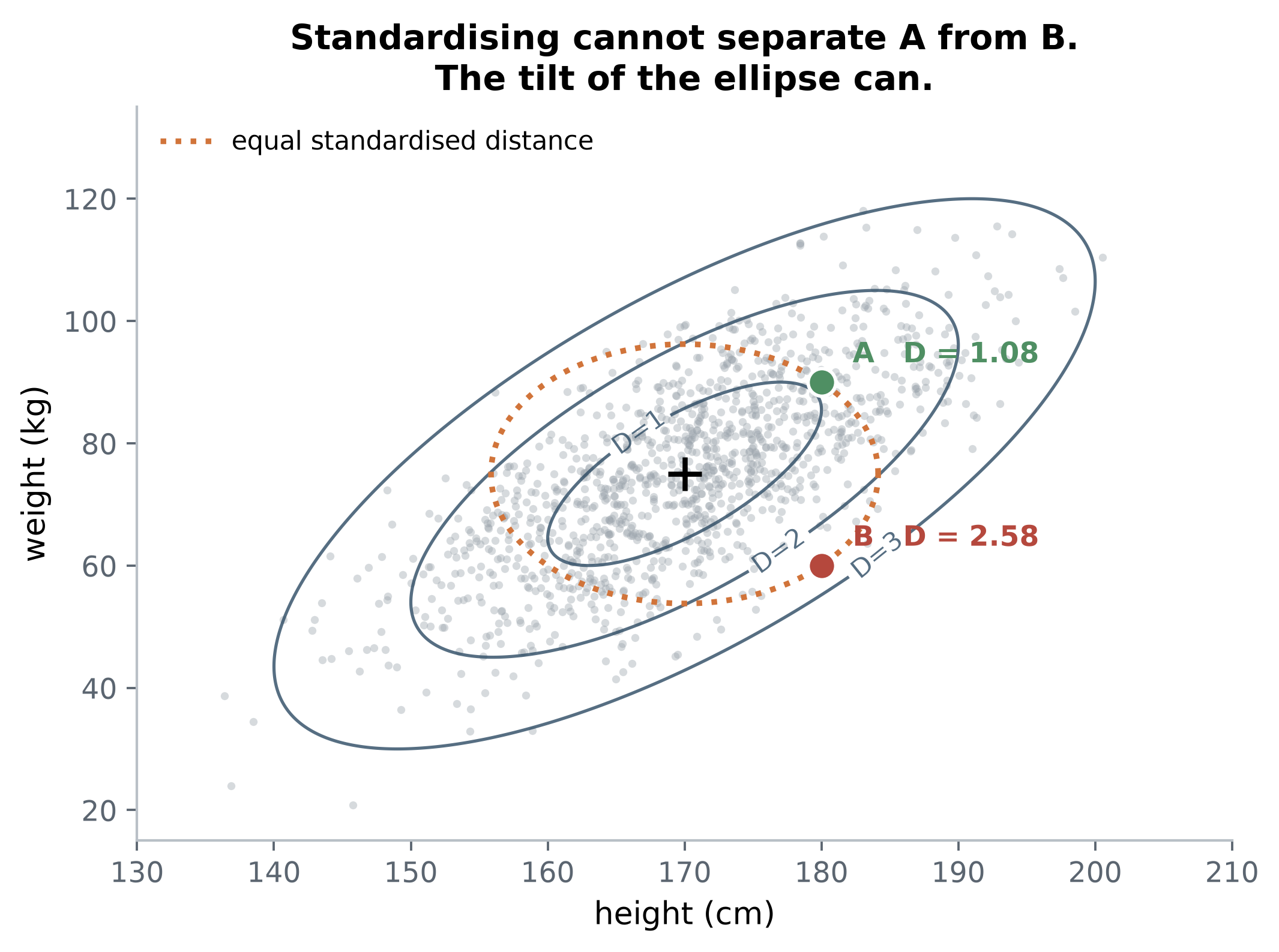
Now consider two people, both aged 50 (exactly average, so age contributes
nothing) and both exactly one standard deviation above average in height:
- **A** is also one SD *above* average weight: `(50, 180, 90)`, tall and heavy.
- **B** is one SD *below* average weight: `(50, 180, 60)`, tall and light.
In raw units both are $(0, +10, \pm 15)$ away from the mean, so their Euclidean
distances are identical. After standardising, both are at $\sqrt{2} = 1.414$.
```{python}
#| label: tbl-two-people
A_person = np.array([50.0, 180.0, 90.0])
B_person = np.array([50.0, 180.0, 60.0])

rows = []
for lab, v in [("A: tall & heavy", A_person), ("B: tall & light", B_person)]:
    d = v - mu_x
    rows.append({
        "person": lab,
        "Euclidean (raw units)": np.linalg.norm(d),
        "Euclidean (standardised)": np.linalg.norm(d / sd_x),
        "Mahalanobis D": np.sqrt(d @ S_inv @ d),
        "Mahalanobis D^2": d @ S_inv @ d,
    })

pd.DataFrame(rows).set_index("person").round(3)
```
::: {.callout-note collapse="true"}
## Maths: where the factor of two comes from
The Mahalanobis distance separates them by a factor of more than two. For two
correlated variables the quadratic form works out to
$$
D^2 \;=\; \frac{1}{1-\rho^2}\Big(z_1^2 \;-\; 2\rho\, z_1 z_2 \;+\; z_2^2\Big),
$$
with $z_j$ the ordinary z-scores. Age drops out because it is uncorrelated,
leaving $z_1 = z_2 = 1$ for A and $z_1 = 1, z_2 = -1$ for B, with $\rho = 0.7$:
$$
D^2_A = \frac{1 - 2(0.7) + 1}{1 - 0.49} = \frac{0.6}{0.51} = 1.176,
\qquad
D^2_B = \frac{1 + 2(0.7) + 1}{1 - 0.49} = \frac{3.4}{0.51} = 6.667 .
$$
The cross term $-2\rho z_1 z_2$ is doing the work.
:::
If a person is taller than average then we expect them to be heavier than
average, since height and weight are positively correlated. The Mahalanobis
distance counts height and weight almost as a single feature, rather than two
separate features.
Being tall and light is unusual. B is represented as far from the centre of
the cloud by the Mahalanobis distance and A is not.
```{python}
#| label: fig-correlation-ellipse
#| fig-cap: "The height–weight plane with contours of constant Mahalanobis distance (solid, tilted). The dotted orange curve is the contour of constant *standardised* Euclidean distance through A and B. It is axis-aligned, and it passes through both points, because standardising alone cannot tell them apart. The tilt is the entire contribution of Σ⁻¹."
#| fig-height: 4.8
S_hw = S_x[1:, 1:]
mu_hw = mu_x[1:]
sample = rng.multivariate_normal(mu_hw, S_hw, 1200)

fig, ax = plt.subplots(figsize=(6.4, 4.8))
ax.scatter(sample[:, 0], sample[:, 1], s=8, color=C["grey"], alpha=0.4, lw=0)

# Mahalanobis contours
gx = np.linspace(mu_hw[0] - 40, mu_hw[0] + 40, 400)
gy = np.linspace(mu_hw[1] - 60, mu_hw[1] + 60, 400)
GX, GY = np.meshgrid(gx, gy)
dd = np.dstack([GX - mu_hw[0], GY - mu_hw[1]])
Dgrid = np.sqrt(np.einsum("...i,ij,...j->...", dd, np.linalg.inv(S_hw), dd))
cs = ax.contour(GX, GY, Dgrid, levels=[1.0, 2.0, 3.0],
                colors=C["dark"], linewidths=1.1, alpha=0.8)
ax.clabel(cs, fmt=lambda v: f"D={v:.0f}", fontsize=9)

# Contour of constant STANDARDISED Euclidean distance through A and B.
# Both sit at sum of squared z-scores = 2, so this is the axis-aligned
# ellipse with semi-axes sqrt(2) * sd in each direction.
sd_hw = np.sqrt(np.diag(S_hw))
th = np.linspace(0, 2 * np.pi, 400)
ax.plot(mu_hw[0] + np.sqrt(2) * sd_hw[0] * np.cos(th),
        mu_hw[1] + np.sqrt(2) * sd_hw[1] * np.sin(th),
        ls=":", color=C["orange"], lw=2.0,
        label="equal standardised distance")
ax.legend(loc="upper left", fontsize=9)

for lab, v, col in [("A", A_person, C["green"]), ("B", B_person, C["red"])]:
    ax.scatter(v[1], v[2], s=95, color=col, zorder=5,
               edgecolor="white", lw=1.2)
    d = v - mu_x
    ax.annotate(f"{lab}   D = {np.sqrt(d @ S_inv @ d):.2f}",
                (v[1], v[2]), textcoords="offset points", xytext=(11, 7),
                fontsize=10, fontweight="bold", color=col)

ax.scatter(*mu_hw, marker="+", s=140, color="black", lw=1.8, zorder=6)
ax.set_xlabel("height (cm)")
ax.set_ylabel("weight (kg)")
ax.set_title("Standardising cannot separate A from B.\nThe tilt of the ellipse can.")
ax.grid(False)
fig.tight_layout()
plt.show()
```
### Redundant columns are not double-counted
Suppose weight gets recorded twice by two related scales, and you
include both columns. Then you add a third related scale, and a fourth.
Standardised Euclidean distance treats each copy as fresh evidence and lets
"weight" dominate the metric. Mahalanobis does not: $\Sigma^{-1}$
records that the copies are redundant, and the squared distance is unchanged
no matter how many of them you add.
That is the metric's main advantage over the obvious alternative, so here it is
measured rather than asserted. Each extra column is a second scale recording
exactly the same weight.
```{python}
#| label: tbl-redundant
#| tbl-cap: 'Adding duplicate weight columns. Standardised Euclidean distance climbs with every copy; $D^2$ does not move. Exact copies make $\Sigma$ singular, so this uses the pseudo-inverse.'
rows = []
for m in range(4):
    sel = [0, 1] + [2] * (m + 1)
    S_m = S_x[np.ix_(sel, sel)]
    Si_m = np.linalg.pinv(S_m)
    dA = (A_person - mu_x)[sel]
    dB = (B_person - mu_x)[sel]
    rows.append({
        "weight columns": m + 1,
        "Euclidean (standardised), A": f"{np.linalg.norm(dA / sd_x[sel]):.3f}",
        "D<sup>2</sup>, A": f"{dA @ Si_m @ dA:.3f}",
        "D<sup>2</sup>, B": f"{dB @ Si_m @ dB:.3f}",
    })
pd.DataFrame(rows).style.hide(axis="index")
```
A and B keep the $D^2$ values they had with one weight column, while the
standardised Euclidean distance to A grows by a factor of
`{python} f"{np.sqrt(4 / 2):.2f}"` across the four rows purely because the
same measurement was recorded four times.
## Categorical features
Everything so far assumed continuous covariates. Categorical ones need one extra
step.
Throughout this section the running example is a fourth covariate alongside
`age`, `height_cm` and `weight_kg`: a **region** with $K = 4$
levels, `north`, `south`, `east` and `west`, occurring with prevalences
$$
p = (0.50,\; 0.30,\; 0.15,\; 0.05).
$$
There is one dominant level, two middling ones, and one deliberately
rare level at 5%, because the rare level is where the interesting behaviour is.
Below, 50,000 units are drawn from it.
If we encode `region` as four indicator (dummy) columns, one per level, this
breaks $\Sigma^{-1}$. Every row of the indicator block sums to exactly one,
which is an exact linear dependency, so $\Sigma$ is singular and cannot be
inverted. With $m$ fully one-hot encoded categoricals the rank deficiency is
$m$, one per block.
There are two standard ways to deal with it, and
they give identical answers.
### Fix A: drop a baseline level
Keep $K-1$ dummies and let one level be the implicit reference. The dependency
disappears, $\Sigma$ becomes invertible, and everything proceeds as normal.
### Fix B: keep all $K$ and use the pseudo-inverse
Keep the full block and replace $\Sigma^{-1}$ with the Moore–Penrose
pseudo-inverse $\Sigma^{+}$:
$$
D^2 = (x - \mu)^{\!\top}\,\Sigma^{+}\,(x - \mu).
$$
$\Sigma^{+}$ inverts $\Sigma$ on its row space and sends the null space to zero.
Since all the centred data already lives in that row space, nothing is lost.
### The two fixes give the same answer
::: {.keybox}
**Fixes A and B are not two approximations to trade off. They give exactly the
same $D^2$, and it does not matter which level you drop.**
:::
The reason: the two encodings hold identical information in different
coordinates (given any three of the four dummies, the fourth is determined), and
$D^2$ is unchanged by any invertible linear reparameterisation of the
covariates. That same property is why you never have to standardise your columns
first, and why centimetres and inches give the same answer.
So pick on convenience.
**Drop a baseline** if you want a well-conditioned, invertible $S$ and
a Cholesky factor you can reuse. This is what you want inside a
rerandomization loop. This is the default I would reach for.
**Use the pseudo-inverse** if you would rather not choose a reference level, if
you are handling several categoricals programmatically, or if $S$ may be
singular for other reasons anyway: more covariates than units, an all-constant
column, a covariate that is an exact linear combination of others. Just set
`rcond` explicitly. See [Practical notes](#practical-notes-and-failure-modes).
Both methods, end to end, for a unit from `west`:
```{python}
#| label: categorical-both-methods
levels = ["north", "south", "east", "west"]
p_true = np.array([0.50, 0.30, 0.15, 0.05])
TOL    = 1e-10                  # never rely on pinv's default; see the notes

region = rng.choice(4, size=50_000, p=p_true)
unit   = 3                      # the unit whose distance we want: 'west'

# ---- Fix A: drop a baseline (north) -------------------------------------
X_a    = np.eye(4)[region][:, 1:]        # south, east, west; north is implied
S_a    = np.cov(X_a, rowvar=False, bias=True)
d_a    = np.eye(4)[unit][1:] - X_a.mean(0)
D2_a   = d_a @ np.linalg.solve(S_a, d_a)

# ---- Fix B: keep all four levels, use the pseudo-inverse ----------------
Dfull  = np.eye(4)[region]
S_full = np.cov(Dfull, rowvar=False, bias=True)     # singular by construction
p_hat  = Dfull.mean(0)
d_b    = np.eye(4)[unit] - p_hat
D2_b   = d_b @ np.linalg.pinv(S_full, rcond=TOL) @ d_b

print(f"Fix A, baseline = north : D^2 = {D2_a:.10f}")
print(f"Fix B, pseudo-inverse   : D^2 = {D2_b:.10f}")
print(f"difference              : {abs(D2_a - D2_b):.2e}")
```
### Mixing continuous and categorical covariates
Nothing special is required: stack the continuous columns and the dummy columns
into one design matrix and take the covariance of the whole thing. The
cross-covariances between the dummies and the continuous columns are estimated
along with everything else, so a categorical that is correlated with age gets
discounted against age automatically.
```{python}
#| label: mixed-design
n_mix = 20_000
region = rng.choice(4, size=n_mix, p=p_true)
# Make region genuinely correlated with the continuous block: shift age by region.
cont = rng.multivariate_normal(mu_x, S_x, n_mix)
cont[:, 0] += np.array([-6.0, 0.0, 4.0, 12.0])[region]

onehot = np.eye(4)[region]
X_full = np.hstack([cont, onehot])            # 3 continuous + 4 dummies (singular)
X_drop = np.hstack([cont, onehot[:, 1:]])     # 3 continuous + 3 dummies (invertible)

unit = np.array([62.0, 180.0, 60.0])          # older, tall, light ...
unit_full = np.concatenate([unit, np.eye(4)[3]])   # ... and from 'west'
unit_drop = np.concatenate([unit, np.eye(4)[3][1:]])

def d2_pinv(X, v, tol=TOL):
    d = v - X.mean(0)
    return float(d @ np.linalg.pinv(np.cov(X, rowvar=False, bias=True), rcond=tol) @ d)

def d2_inv(X, v):
    d = v - X.mean(0)
    return float(d @ np.linalg.solve(np.cov(X, rowvar=False, bias=True), d))

print(f"full one-hot + pseudo-inverse : {d2_pinv(X_full, unit_full):.8f}")
print(f"baseline dropped + inverse    : {d2_inv(X_drop, unit_drop):.8f}")
print(f"continuous columns alone      : {d2_inv(cont, unit):.8f}")
```
The first two agree, as they must. The third is smaller, which is the point: it
is the distance that ignores the fact that this person also comes from the
rarest region.
## Practical notes and failure modes
**Singular or ill-conditioned $S$.** With $p$ close to $N$, exact collinearity,
or full one-hot encodings, $S^{-1}$ does not exist. Use $S^{+}$ with an explicit
tolerance, or drop columns until it is invertible. Watch `np.linalg.cond(S)`:
once it passes roughly $10^{10}$, $D^2$ is being driven by directions in which
the data barely varies, and those directions are usually noise.
**Redundancy is free, but only statistically.** Adding correlated covariates
does not upweight them. It does worsen the conditioning of $S$, and it raises
$p$, which matters as soon as you start comparing $D^2$ against a $\chi^2_p$
reference.
**Set your own tolerance on `pinv` and `matrix_rank`.** A one-hot covariance has
an eigenvalue that is exactly zero in theory, but floating-point arithmetic
returns something around $\pm 10^{-16}$ instead. NumPy's default cutoff is
relative to the largest singular value and is tight enough that this
structurally-zero eigenvalue is not reliably discarded:
```{python}
#| label: pinv-tolerance
#| code-fold: true
print("eigenvalues       :", np.round(np.linalg.eigvalsh(S_full), 18))
print("smallest, in full :", f"{np.linalg.eigvalsh(S_full)[0]:.3e}")
print()
print(f"matrix_rank, default tol : {np.linalg.matrix_rank(S_full)} of 4   <- wrong")
print(f"matrix_rank, tol=1e-10   : {np.linalg.matrix_rank(S_full, tol=TOL)} of 4   <- right")
```
Whether it bites depends on exactly where that eigenvalue lands, which varies
with the data. On this particular matrix `pinv` happens to be fine, but
`matrix_rank` already reports a singular matrix as full rank. The failure mode
for `pinv` is worse than for `matrix_rank`, because it is silent: you get a
plausible number that is quietly wrong rather than an obviously wrong integer.
Pass `np.linalg.pinv(S, rcond=1e-10)` and `matrix_rank(S, tol=1e-10)` as a
matter of habit, or sidestep both by dropping a baseline.
**Rare categorical levels dominate the metric.** Assuming that the categorical
block is uncorrelated with every other column, a single unit's squared distance
from the centre, from its level membership alone, is
$$
D^2 = \frac{1 - p_k}{p_k},
$$
which grows without bound as the level gets rarer:
| prevalence $p_k$ | 50% | 10% | 5% | 1% |
|---|---|---|---|---|
| $D^2$ | 1 | 9 | 19 | 99 |
| $D$ | 1 | 3 | 4.4 | 9.9 |
At $p_k = 0.01$, belonging to that one level puts a unit as far from the centre
as a continuous covariate sitting **ten standard deviations** from its mean.
Collapse levels below a few percent into an `other` category, or the metric
quietly becomes a metric about that one level.
**Every covariate is treated as equally important.** $D^2$ is invariant to
rescaling, which is a virtue for units and a limitation for priorities. It has
no way to include that the baseline outcome measurement matters more than the
recruitment site.
**Outliers inflate $S$.** The covariance is estimated from the same data you are
measuring against, so a handful of extreme units widen the ellipse and make
everything look closer to the centre than it is. Look at your covariates before
trusting the metric.
## References
- Mahalanobis, P. C. (1936). On the generalised distance in statistics.
*Proceedings of the National Institute of Sciences of India*, 2(1), 49–55.
- Rubin, D. B. (1976). Multivariate matching methods that are equal percent bias
reducing. *Biometrics*, 32(1), 109–120.