Pairwise matching
matching
design
inference
Pairing units before you randomise: when it beats rerandomization, why the pairing has to be solved properly, and how to analyse the result.
Consider running an experiment with a few hundred participants. Before the intervention begins, you’d like to split them into a control group and a treatment group that are as similar to each other as possible. Rerandomization reaches that by trying ordinary random splits and keeping only the most balanced one. Pairwise matching works by pairing units with similar characteristics, and within each pair, randomly deciding which unit receives treatment and which serves as its control. So the two groups are balanced pair by pair, not just on average.
This article asks whether matching beats rerandomization, how to pair the units, and how to analyse the experiment afterwards.
What it does
Closeness between two units is measured with the Mahalanobis distance. With (even) \(N\) units and \(k\) covariates:
- Compute the covariate covariance matrix \(S\) once, from all \(N\) units.
- For every pair of units \(i\) and \(j\), compute the squared distance between them: \[ D^2(i,j) \;=\; (x_i - x_j)^{\!\top} S^{-1} (x_i - x_j). \]
- Choose the \(N/2\) pairs that minimise the total within-pair distance, subject to covering every unit exactly once.
- Inside each pair, randomly assign one unit to treatment and one to control.
We will cover the case where \(N\) is odd later in this article.
Step 2 is the same quadratic form as in the Mahalanobis article, applied to the gap between two units instead of the gap between a unit and the mean.
Step 4 is what keeps this a randomised experiment. If we assigned deterministically inside pairs, e.g. the higher-spending unit always becomes the control, there would be a single possible split and no basis for a \(p\)-value, whereas the random assignments leave \(2^{N/2}\) possible splits, about \(1.6 \times 10^{60}\) at \(N = 400\).
Does it gain more than rerandomization?
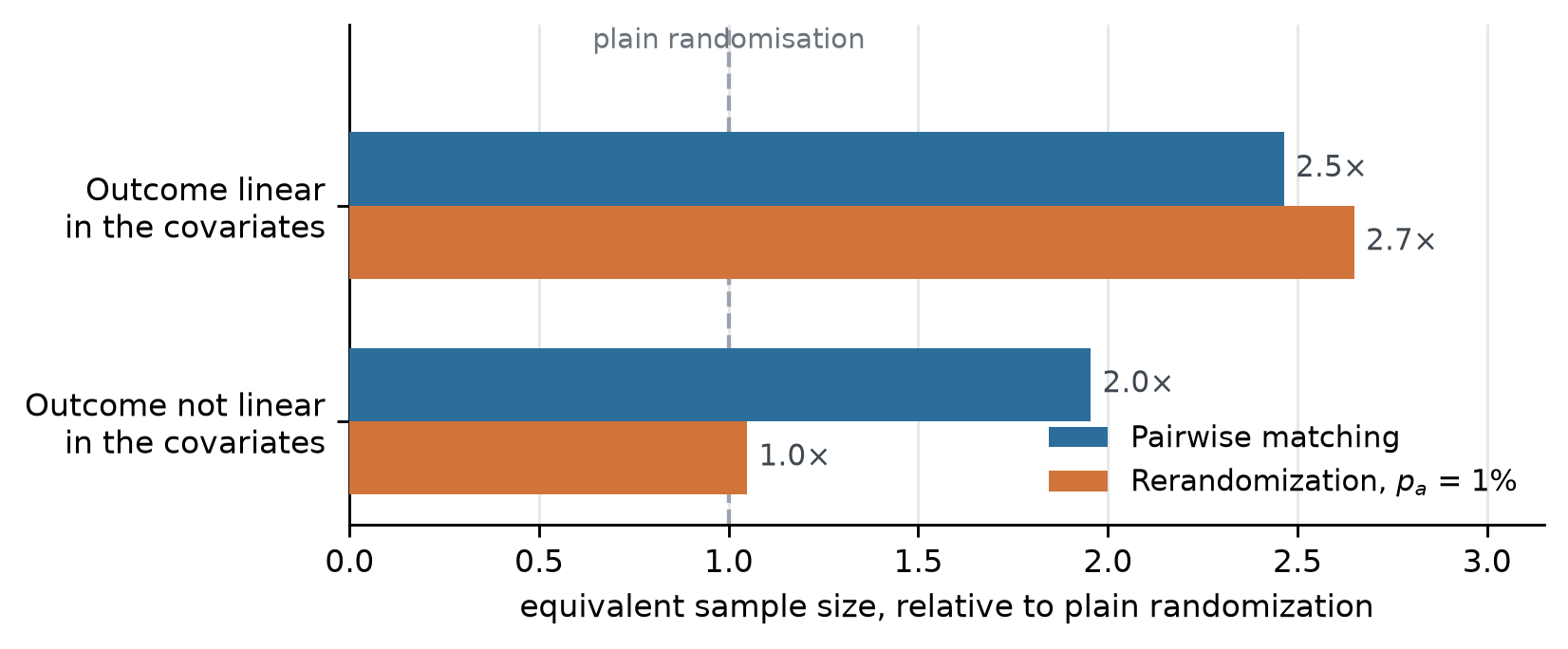
The plot below shows the results for an experiment with 400 units and four covariates. These “X” predictor values are kept fixed, but two “y” outcomes are built on X, differing in how much of the outcome a linear function can predict. Pairwise matching and rerandomisation are then run 4,000 times against each outcome. Matching solves the optimal pairing once and then randomly assigns treatment within each pair, so its 4,000 assignments are all different. The gain is expressed as the sample you would need under plain randomization to estimate the treatment effect just as precisely.
The two designs behave similarly on a linear outcome and differently on a non-linear one. Rerandomization will keep the difference in covariate means low, but is limited by how much of the outcome is linear in the covariates. That falls from 0.64 to 0.06 between the two rows, and the bar collapses with it.
Matching is limited by the relationship between the covariates and the outcome. If two units in a pair sit close together in covariate space, and this makes it more likely that their outcomes will be similar, then it doesn’t matter if the relationship is linear or not, the pairing will be effective. But if there is no relationship then matching will deliver no gain. The two rows of the figure above assume that there is a relationship.
What it is worth on two real datasets
Every number above comes from generated covariates and outcomes. I’ll now look at two real datasets.
With LaLonde’s National Supported Work data, the measured \(R^2\) is only 0.04. So there’s no point spending effort on the design here: the optimal matching is worth 2% more data. So pairwise matching is not a magic bullet that can make sample sizes sufficiently large. For Project STAR (Student/Teacher Achievement Ratio) data, pupils’ grade-two reading and maths scores could be used to predict their grade-three reading scores, with \(R^2\) equal to 0.65. In this setting, the pairwise matching would be worth 3.0 times the sample.
Technically, the equivalent sample size under pair randomization is \(1/(1-\rho)\), where \(\rho\) is the within-pair correlation of the outcome. STAR’s matching beats the 2.9\(\times\) that \(1 - R^2\) would allow. \(R^2\) measures the linear share.
NoteChecking both numbers against theory
The variance ratio under rerandomization is \(1 - (1 - v_a)R^2\), with \(v_a\) the shrinkage factor from the rerandomization article and \(R^2\) the linear one. At \(k =\) 4 and \(p_a = 1\%\), \(v_a =\) 0.049, so the formula predicts a variance ratio of 0.39 for the linear model against 0.38 measured, and 0.94 for the non-linear model against 0.95 measured. Splitting the outcome into its linear fit and the residual shows the mechanism directly: under rerandomization the variance of the fitted part shrinks by a factor of about \(v_a\), and the variance of the residual part does not move.
For matching, a perfectly matched sample would reduce the variance to \(1 - R^2 =\) 0.36 here against 0.51 achieved. The shortfall is the price of pairs that are close but not identical.
The two designs also differ in what you can do about a disappointing number. Tightening the threshold drives \(v_a\) towards zero, so rerandomization has a dial to turn.
TipWhich to reach for
Matching is the safer default because it works even when the relationship between covariates and outcome is complex. Rerandomization is easier from an administrative perspective because you don’t have to keep track of the pairing, which sometimes cannot survive to the analysis stage.
The pairing is an optimisation problem, not a sorting problem
The gain above assumes the pairing is solved optimally.
The obvious way to form pairs is the “greedy” approach: pair the two closest units anywhere in the sample, then repeat on what is left. It is easy to explain and implement, but it does not produce the optimal pairing.
You can drag the slider to watch it choose. The middle plot shows what each pair costs, on a log scale because the range is wide, and the bottom panel shows the running total. Each plots the optimal matching alongside, both ranked closest pair first. The early pairs are nearly free, and the final one costs 21.0 against 6.6 for the other nineteen put together.
drag to add pairs
Greedy matching is closer than the optimal matching on 12 of the 20 ranks, because taking the nearest available pair at every step collects near-duplicates that the optimal matching gives up. Those wins come to 0.8 in total, against 20.5 at the ranks where it loses.
Greedy pairing strands the units it leaves until last. The gap for those last pairs goes into the variance of the treatment effect estimate, so the tail of the distance distribution matters more than its total.
NoteWhat the lengths mean here, and what they would mean on real data
Here the sample is rescaled so that \(S\) is the identity. The Mahalanobis distance is then the plain straight-line distance, so each line’s length is exactly what is being minimised. Real covariates are usually correlated. Then equal distances form tilted ellipses rather than circles, so screen length no longer tracks distance. The Mahalanobis distance makes a gap along the long axis cheap, while the same gap across the short axis is expensive because that combination is rare.
In the 40-unit example above, the greedy algorithm reaches 3.5 times the optimal total distance and the cost of the worst pair is 11 times greater. The table below runs the same comparison for different sample sizes and numbers of covariates.
| Sample | Total D2, optimal | Total D2, greedy | Worst pair, optimal | Worst pair, greedy |
|---|---|---|---|---|
| N = 100, k = 4 | 63.0 | 82.1 (+30%) | 5.47 | 10.41 (1.9×) |
| N = 200, k = 4 | 78.5 | 113.2 (+44%) | 4.70 | 14.80 (3.1×) |
| N = 200, k = 8 | 409.1 | 505.0 (+23%) | 10.20 | 54.08 (5.3×) |
The two columns move in opposite directions as the sample grows. At \(N = 200\) with four covariates greedy’s total is only 44% above optimal, against 253% at 40 units, so the totals converge. Its worst pair still costs 3.1 times more, and at 8 covariates 5.3 times more. The total becomes a worse and worse guide to the thing that matters.
Edmonds’ blossom algorithm solves the problem exactly in \(O(N^3)\). Because any unit may pair with any other, the graph is not bipartite and the Hungarian algorithm does not apply; Greevy et al. (2004) introduced this non-bipartite form for the design. In Python it is available in networkx and in R through the nbpMatching package. The button in the bottom right shows the optimal matching for comparison.
Odd numbers, and units with nothing close to them
One mechanism can actually solve two awkward cases. A perfect matching needs an even \(N\), so an odd sample leaves a unit over. Separately, a sample may contain units that sit far from everything else, and forcing them into pairs produces high-variance assignments.
Both are solved by adding sinks. A sink is a phantom unit placed at distance zero from every real unit, with no edge to another sink. Because a sink has to be matched and cannot take another sink, it takes a real unit out of the experiment. Pairing with a sink is free, so the solver spends its sinks on whichever units were most expensive to pair.
One sink absorbs the outlier unit in an odd sample. Beyond that, sinks come in pairs: each one removes a real unit, so you need an even number of them to leave an even number of units behind. Adding two sinks excludes the two units whose matches would have been worst, four excludes the worst four, and so on.
Drag below to add sinks to a sample containing four units placed well away from the rest.
02468
The first two sinks remove the two worst-placed units and the worst remaining pair falls by 64%. Two more remove the rest of the awkward group. After that the returns shrink, and every further sink costs real sample size.
Analysing a matched experiment
The point estimate of the gap between the treatment and control groups is the same whether you use a two-sample t-test or analyse the within-pair differences.
If you treat the control and treatment groups as independent, a two-sample \(t\)-test would compute the standard error from the within-arm variances. The interval comes out 40% too wide, and covers the true effect 99.3% of the time instead of 95%.
Differencing within pairs fixes it. The within-pair difference is the unit of analysis, and its spread already reflects how closely the pairs were matched, so the interval lands at 94.9% coverage. Equivalently, a regression of the outcome on treatment plus a fixed effect for each pair is the same calculation, and gives the same standard error. The cost is degrees of freedom, \(N/2 - 1\) rather than \(N - 2\).
A conservative interval is not always a safe one
Lost precision is not the only consequence of using an interval that is too wide.
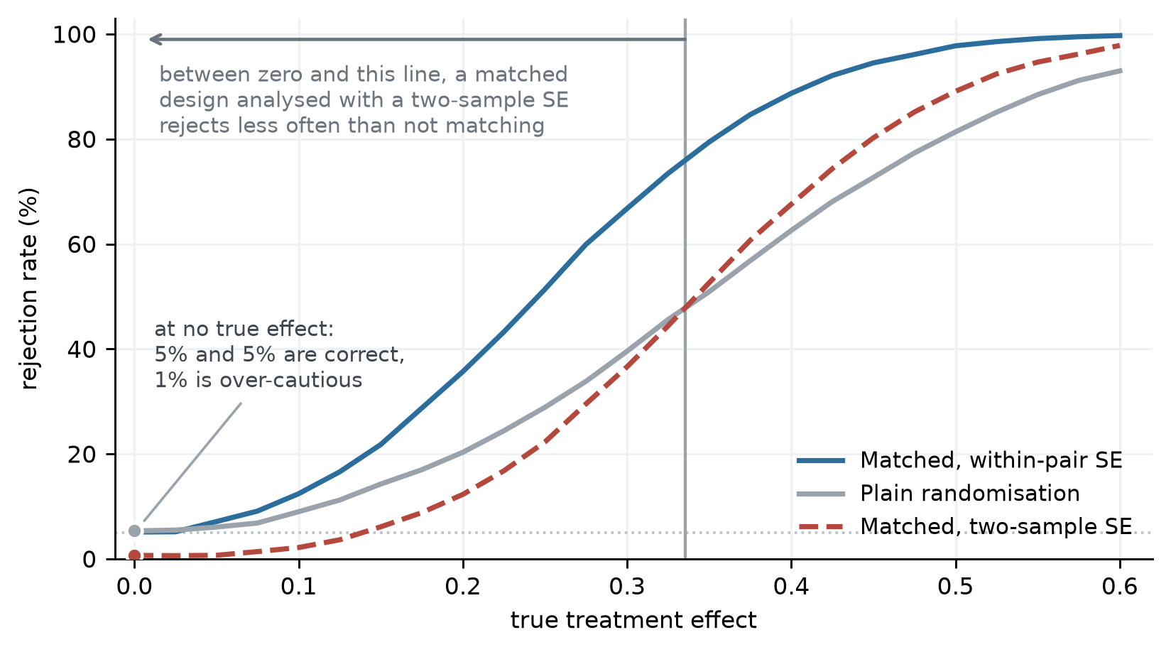
The matched design analysed with a two-sample standard error (dashed red line) rejects less often than plain randomisation (grey line) does for small effect sizes. At a true effect of zero the test is miscalibrated in the safe direction: you tolerate a 5% false positive rate and get 0.7%. And when the effect is greater than zero it is lost power. Bruhn and McKenzie report that failing to account for the randomisation method gives tests of the wrong size, and can give less power than a plain random draw would have. The matched, within-pair SE method (blue line) is what the design was for.
WarningThe pairing has to survive to the analysis
You need to make use of the pair labels in the analysis stage to fully gain from the matching.
TipWhat to do
Pair on the covariates you have reason to believe predict the outcome, solve the matching exactly, keep the pair identifier, and analyse within pairs. Matching on covariates that do not predict the outcome spends degrees of freedom and returns nothing.
References
- Bruhn, M. and McKenzie, D. (2009). In pursuit of balance: randomization in practice in development field experiments. American Economic Journal: Applied Economics, 1(4), 200–232.
- Dehejia, R. H. and Wahba, S. (1999). Causal effects in nonexperimental studies: reevaluating the evaluation of training programs. Journal of the American Statistical Association, 94(448), 1053–1062. Source of the National Supported Work sample used here.
- Edmonds, J. (1965). Paths, trees, and flowers. Canadian Journal of Mathematics, 17, 449–467.
- Krueger, A. B. (1999). Experimental estimates of education production functions. The Quarterly Journal of Economics, 114(2), 497–532. Project STAR, the source of the grade-three sample used here.
- LaLonde, R. J. (1986). Evaluating the econometric evaluations of training programs with experimental data. The American Economic Review, 76(4), 604–620.
- Greevy, R., Lu, B., Silber, J. H. and Rosenbaum, P. (2004). Optimal multivariate matching before randomization. Biostatistics, 5(2), 263–275.
- Lu, B., Greevy, R., Xu, X. and Beck, C. (2011). Optimal nonbipartite matching and its statistical applications. The American Statistician, 65(1), 21–30.
- Morgan, K. L. and Rubin, D. B. (2012). Rerandomization to improve covariate balance in experiments. The Annals of Statistics, 40(2), 1263–1282.